Whether you are doing keyword research for SEO or text analysis for other purposes, Excel can be very handy if you implement some tricks that I am going to share with you in a set of posts called “Keyword research in Excel”.
In this post we are going to cover one of the basic concepts of keyword research – keyword grouping.
Why is keyword grouping important?
When you are doing keyword research for SEO the output of this research will be a keyword map which essentially is a list of keywords and their search volumes, grouped by certain topics of interest. Of course, there are always several predefined topics, but most important topics are usually discovered during the research itself. And that’s why we need grouping – to define topics with the best combinations of keywords and their respective search volumes.
Think of the following grouping examples: branded keywords, locality (city, region), year, transactional, informational.
Preparing and cleaning the data.
First things first. In any tasks related to large amounts of data the most important thing is properly prepared and clean data. We already have several spreadsheets with various keywords. After we combine them in a single list with columns Keyword, Search Volume and Competition here’s what we are going to do:
1. Make a “smart table” out of this list by clicking on any cell in your list and pressing CTRL+T on your keyboard (or go to the top menu Insert → Table).
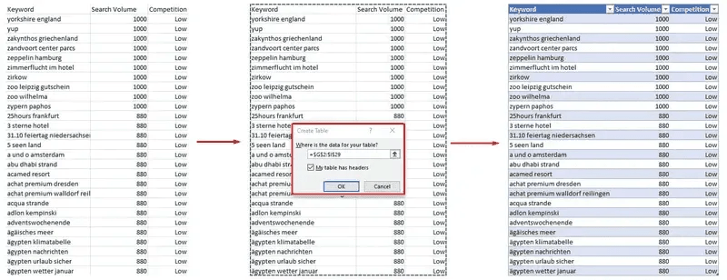
You will see that Excel automatically detected the whole list and selected all required cells. If that didn’t happen then select manually the whole range and then repeat table creation.
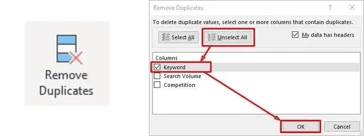
2. Remove duplicate keywords from your table. Click on any cell in your table and go to the top menu Data → Remove duplicates.
In the new popup window unselect all columns by pressing the “Unselect All” button and then select only the Keyword column and press “OK”.
Basic grouping: word count and search volumes.
Now you are ready to start grouping your keywords. Let’s do some basic grouping: by the number of words in a phrase and by search volumes.
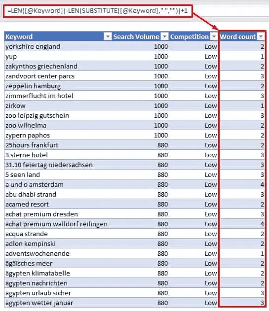
As there is no default formula to count words in a single cell, what we are going to do now is to calculate the number of spaces between words (if any).
Here’s a formula to do that:
=LEN([@Keyword])-LEN(SUBSTITUTE([@Keyword],” “,””))+1
Grouping by search volume is possible with a number of nested IF statements. We just need to define the bucket size. Let’s use the following buckets / groups:
- Below 100
- 100-499
- 500-999
- 1000+
Here’s a formula for this kind of grouping:
=IF([@[Search Volume]]<100,”0-100″,IF([@[Search Volume]]<500,”100-499″,IF([@[Search Volume]]<1000,”500-999″,”1000+”)))
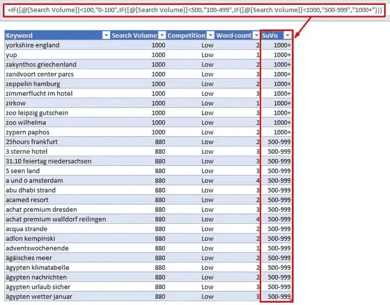
Note that in case of nested IF statements the order of nesting formulas is important: Excel calculates such formulas from left to right, meaning that the very first condition will be checked first, if the condition is not met, then the second condition will be checked, then third and so on. In our case if we put the “<1000” condition in the first place, then we wouldn’t see the first two groups.
Advanced grouping: using additional tables to automate formulas.
The example with nested IF statements is actually the one we are going to pimp up now in order to do the advanced grouping. We are also going to utilize the Total Row functions of our “smart tables”.
Let’s have a brief look at what a Total Row of a “smart table” is.
![A desktop screenshot of Microsoft Excel illustrating how to use table summary options. At the top ribbon, the "Table Design" tab is highlighted with a red box. A red line points to the "Total Row" checkbox, which is checked.
Another long red arrow extends down from that setting to the actual total row at the bottom of the data table, focusing on a cell displaying the value "24960". A dropdown menu is active for this cell, showing that "Sum" is selected. Above the table columns, the formula bar displays the corresponding Excel function: =SUBTOTAL(109,[Search Volume]).](https://digital-loop.com/uploads/2026/06/keyword-number-calculation-3.56d45b09.png)
Total Row, when enabled, offers a number of calculations that it can make for each column: count rows, sum numbers, show minimum or maximum value, etc. It is also possible to use other built-in Excel functions. The best thing about the Total Row is that it works independently of the “smart table” size, i.e. no matter if there are 5 rows or 5000 rows it will execute the same calculation. So, knowing all that we are going to use the Total Row to quickly create multiple IF conditions for our advanced grouping with the REPT (repeat) function.
Take a look at the example below.
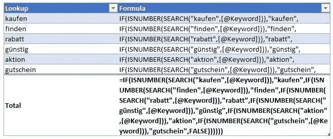
4Here you see a table with two columns: Lookup and Formula. First column is for manual input only. The Formula column automatically creates an IF condition that we’re going to use further. It just takes the value of the Lookup column and concatenates it with other text elements to make a formula string out of it. In other words, the results of the formulas in this column are other formulas (perceived by Excel as text strings for now).
Here’s the formula that takes values and concatenates them:
=”IF(ISNUMBER(SEARCH(“””&SUBSTITUTE([@Lookup],” “,”*”)&””””&”,[@Keyword]”&”)),”””&[@Lookup]&”””,”
And here’s the result of that formula:
IF(ISNUMBER(SEARCH(“seo”,[@Keyword])),”seo”,
You can now see a number of IF conditions in that column for each row. And yes, there is no error – the closing parentheses were skipped on purpose. But how do we combine all of that in a single formula? Well, the magic happens in the Total Row where we use the following formula to concatenate all IF conditions in a single long string:
=CONCAT(“=”,[Formula],FALSE,REPT(“)”,COUNTA([Formula])))
What this formula does is that it takes all values from the Formula column and concatenates them into a single string. It also adds a “=” symbol and adds closing parentheses, so that the resulting string looks exactly like an Excel formula should look like.
There are two limitations, however, in Excel, that you have to know about.
The first one is that the maximum number of nested IF statements in a formula is 64 which means that for a single column with keyword groupings we may use not more than 64 different keywords. That’s why, for example, in a keyword analysis with geographical grouping by city one would require two such columns for cities in Germany with a population of 100.000+ people.
The second limitation is Excel’s formula length. It may not exceed 8.192 symbols. This limitation never affected my most complex formulas, but still it exists.
Implementing grouping rules.
Ok, so what do we do now with all these columns, rows and formulas?
- Copy the resulting cell of the Formula column in our Total Row.
- Switch back to our Keyword table and paste copied data as “Values only” (to do so press CTRL+ALT+V and choose “values” in the menu).
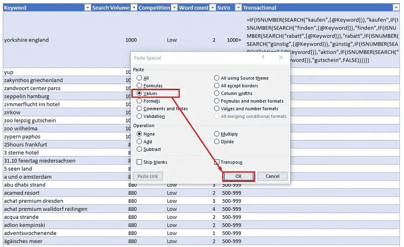
- Press F2 to enter the cell and then press ENTER.
After that the formula will no longer be perceived as a text string, but as an actual formula. That’s why it will start working immediately and you will see the results of grouping defined by the conditions we used.
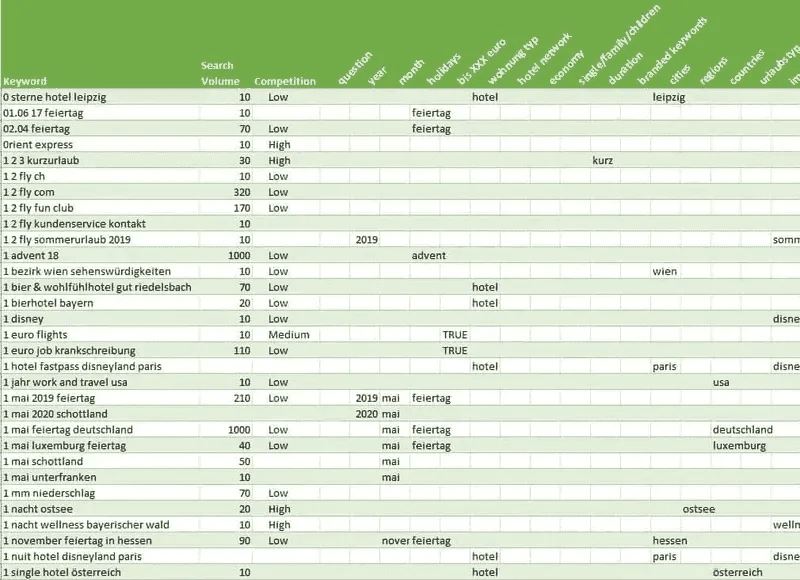
![A desktop screenshot of an Excel spreadsheet data table with columns labeled "Keyword", "Search Volume", "Competition", "Word count", "SuVo", and "Transactional".
At the top, a large red box outlines the nested master formula used for the column: =IF(ISNUMBER(SEARCH("kaufen",[@Keyword])),"kaufen",IF(ISNUMBER(SEARCH("finden",[@Keyword])),"finden",IF(ISNUMBER(SEARCH("rabatt",[@Keyword])),"rabatt",IF(ISNUMBER(SEARCH("günstig",[@Keyword])),"günstig",IF(ISNUMBER(SEARCH("aktion",[@Keyword])),"aktion",IF(ISNUMBER(SEARCH("gutschein",[@Keyword])),"gutschein",FALSE)))))). A red arrow points from this formula box directly down to the "Transactional" column, which is completely enclosed in a red rectangular frame.
While most rows in this column return FALSE, one specific row is highlighted with red underlines to demonstrate the formula working: the keyword "zoo leipzig gutschein" triggers the nested check, successfully returning the value "gutschein" in the transactional intent column.](https://digital-loop.com/uploads/2026/06/keyword-number-calcuation.8567444a.png)
Here’s an example of how a table with several grouping conditions may look like:
Knowing this trick you can make keyword grouping a much easier task. Just make several copies of such “smart tables” – one for each grouping type and simply type text strings that you assume appear in your keywords. Then copy resulting formulas from the Total Row to your keyword table and enjoy!
Bonus!
To make your life even easier we created a downloadable Excel file with grouping table templates that you can use for your keyword research.
The file contains an improved grouping table with an additional Topic column, that helps defining several related subtopics in a single grouping rule (for example, if you want to group different BMW car models in a single group with subgroups like “X3”, “X5”, “i3” and so on).